Weeks lab advice for making figures in IDL

Introduction

We frequently make figures and often need to make nice figures. Usually this starts with making figures for a presentation, and eventually we make figures for a publication -- often starting with a previous version of the figure make for a presentation. You are welcome to use any program you like to make your figures. That being said, if you want to use IDL to make your high-quality figures, this page will explain how to do so. Advantages of using IDL:

• Your data may well already be in IDL format.
• You have access to the full functionality of IDL to further process your data, as needed. Want to fit your data to a line? To a polynomial? Use IDL's built-in linfit and poly_fit. Want something fancier? Just code it up!
• When you are working on figures for a publication, I will have lots of comments for revision. It is helpful if you can easily modify your figure in small ways:
  • Changing font sizes by small percentages up or down.
  • Changing colors of lines or symbols.
  • Changing the thickness of lines.
  • Changing shapes of symbols.
  • Writing text in arbitrary locations. We often follow the David Weitz advice of avoiding a legend, and instead, just labeling each curve directly. (Examples below.)
  • Writing text at arbitrary angles on your graph. For example, labeling a fit line "slope = 1.5".
  • Labeling an axis with text such as 0, pi, 2 pi for a graph related to angles.
• IDL lets you specify your figure with a text file, so it's easy to make small adjustments -- no mouse dragging / fiddling.
• That text file is a great permanent record of how you made the figure. The method described on this webpage keeps your data, the figures, and the files to make your figures in the same directory on a lab Linux computer. This is really helpful if someone needs to reconstruct your figure for some reason in the distant future.
• IDL lets you save your graph as a PostScript file, which is a format that does vector graphics. This means your graphs will always be displayed at the highest resolution possible whether printed out or on a computer screen. Or to quote directly from Wikipedia, "the user can resize the image infinitely without losing any quality." If you want to use another program for publication-quality graphs, I'm going to insist you get that program to produce either PostScript or PDF (another vector graphics format).
• IDL also lets you save your graph as a JPEG. In fact, using the IDL script discussed below, you get the PostScript and JPEG at the same time. Thus you can easily import your graph into a presentation program such as PowerPoint.

• There's a learning curve, so if you already know some other plotting program you might not want to change.
• For quick plots, there might be faster ways. For example, some people prefer to have their data in Excel and use Excel's built-in graphing tools. (Or Google Sheets, or OpenOffice on linux.)

The script

IDL> @mkfigure

• The script puts your graph in a PostScript file.
• It also converts that PostScript file to JPG so you have both a PostScript file and a JPG file when you're done.
• It changes from the default IDL font to Times, which is much preferred for high-quality figures.
• The script also loads in a color palette I quite like which I've seen called "a less angry rainbow" or "cubehelix rainbow." Some info here and here. I can't find the original page where this rainbow first appeared.

Just imagine how nice your graphs will look using colors from this palette!

mkfigure -- download the script here. Or, on any of our lab Linux computers, the script is located at /data/eric/mkfigure.sh . The letters "mk" stand for "make."

How to use:

1. Copy the script to the directory where you want your figure to be made.
2. Rename the script, usually with a name related to the figure you want to make, like "mkmsd" or "mktrajectories".
3. Edit the first line of the script to provide a filename for your figure, for example "msd" or "trajectories".
4. Put your plot commands between the lines marked "BEGIN PLOTTING BELOW" and "END PLOTTING ABOVE". Often you start by putting plotting commands you were already doing in IDL to make a simpler version of the graph.
5. Try running your script. It will display an image of your figure. As needed, look at the last two lines of the script. One line displays a fullsize image of your figure, the other halfsize. Uncomment the one you desire. In other words, if your figure ends up looking too big on the screen, just uncomment the smaller version. And vice versa.
6. Do not otherwise edit the lines at the top or bottom of the script unless you know what you're doing.
7. One possible exception: the line with the linux command "pstopnm" sets the resolution of your JPG file, so as described in a comment in the 'mkfigure' file, you can change this line to increase your resolution. (Or decrease it, although I'm not sure why you'd want to do that.)

Helper files

• all.zip -- zip file containing all of these files listed below, along with 'mkfigure'
• bbox_add.pl -- linux script -- I think the original version is here.
• pagebbox.sh -- linux script written by me
• cropjpg.pro -- IDL program written by me
• ericcol.tbl -- IDL color table file where color tables 75 - 80 are made by me.
  The script uses color table 76, which is the rainbow along with color 0 = black. If you need darker colors, use color table 77; light colors are in color table 79. And when I say "use color table 7" I mean change '76' to '77' in the the sixth line in the 'mkfigure' file where I load color table 76.
• ktex2idl.pro -- IDL program written by Ken Desmond (perhaps based on IDL's tex2idl.pro?)

Setup file

My preferred method is to have a separate IDL script called "setup" that reads in data for the figure(s) I want to make. The concept is that reading in files causes wear & tear on the hard drive, and also takes time. So just read in these files once. Perhaps also, do any pre-processing of the files, especially if it's time intensive. And then the plotting is put into the "mkfigure" script, that is, the plotting of the data you read in and/or processed in "setup".

This is especially useful when you are making a series of minor changes to the "mkfigure" file to make your figures look amazing. You don't want to keep reading in the data every single time. That's really the reason I keep "setup" and "mkfigure" as separate files. Often for a given project (or paper) I will have just one "setup" file in the directory containing the data for that project, and that file will read in data for any and all figures I'm making. Then I'll have separate files starting with "mk" that make the various figures related to that project.

Examples

Introduction

If you're on a lab linux computer, all of these can be found in /data/eric/figures/ . Go there and try running the scripts as suggested below! Otherwise, you can download the setup & mkfigure files, along with the necessary data, in examples.zip.

This is Fig. 3 from Tapia-Ignacio et al., PRE 102, 022902 (2020). On the lab Linux computers, you can make this with IDL> @setup01 IDL> @mkfig01 Comments: The script uses the graphics keyword POSITION to draw the three graphs at different locations on the screen. After the first graph is drawn, the second and third graphs also use the graphics keyword /NOERASE to avoid clearing the screen. With POSITION you have to specify the lower-left corner and the upper-right corner of the graph. These specifications have to be between 0 and 1, that is, you're giving coordinates relative to the screen where (1,1) is the upper right hand corner of what's possible to plot. My usual trick for multi-panel graphs is to define some variables to make this easier. For this three panel graph, I have: x1 = 0.10 & x2 = 0.35 y1 = 0.05 & dy = 0.20 y2 = y1 + dy + 0.02 y3 = y2 + dy + 0.02 Panel (a) is then POSITION=[x1,y3,x2,y3+dy] and (c) is POSITION=[x1,y1,x2,y1+dy]. The advantage of this is that if I want to make the graphs slightly wider or narrower, I just change x2 near the top of the plotting commands. To make all the graphs slightly taller, I increase 'dy'. Changing the space between the graphs would be changing the '0.02' in the last two lines. If I decided I needed a fourth panel, it would be straightfoward to add in a 'y4' and reduce 'dy' and maybe 'x2' to make the graphs all a bit smaller. Likewise each graph is made using CHARSIZE=cs where the variable 'cs' is set near the top of the script, so I can adjust the font size of all three panels simultaneously. In this script I also use the same CHARSIZE for the (a) (b) (c) labels, although for some figures I want those to be a different size so I might use a variable 'cs2' for that size. The IDL command XYOUTS is used to label the curves with their alpha values in panel (a), and also used to add the panel labels (a) (b) (c). In panel (c), I use a small for-loop to add the error bars by drawing horizontal and vertical lines at the appropriate places. I use Ken Desmond's program "ktex2idl.pro" to label the axes -- in other words, to get subscripts and superscripts, math symbols like alpha, etc. In panel (c) I use YRANGE=[2,20] and /YSTYLE to force the vertical axis to be between 2 and 20, rather than letting IDL go with its preference of 1 to 100. This figure uses advice I got from Harry Swinney: the two most opposite symbols (and thus easiest to distinguish) are circles and triangles.

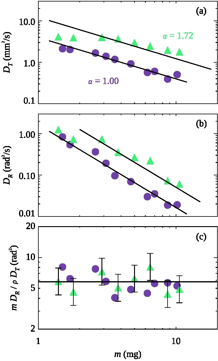
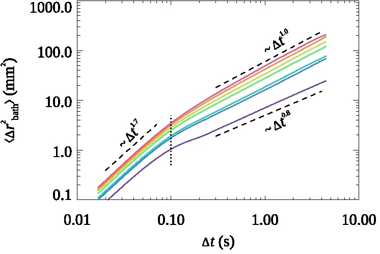
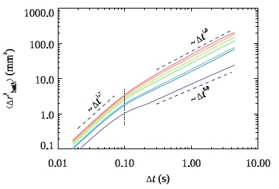
This is Fig. 4 from Tapia-Ignacio et al., PRE 102, 022902 (2020). On the lab Linux computers, you can make this with IDL> @setup02 IDL> @mkfig02 Comments: The dashed lines are labeled with XYOUTS using the ORIENT keyword to rotate the text. For example: xyouts,0.03,1.0,orient=45,ktex2idl('\sim$\Delta{}t$^{1.7}'),chars=cs,/data Here I'm making full use of the rainbow color palette. This graph is just one panel so I did not use POSITION to try to resize it.

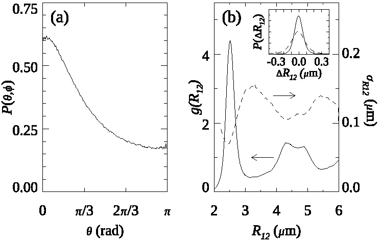
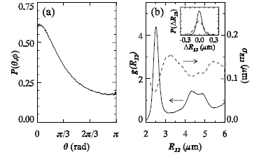
This is Fig. 4 from Weeks & Weitz, PRL 89, 095704 (2002). On the lab Linux computers, you can make this with IDL> @setup03 IDL> @mkfig03 Comments: This is old school, just black & white! It's also old school in that it predates "ktex2idl", so the math symbols are done using IDL's built-in font-changing commands. For example, the vertical axis of panel (a) is labled "!8P!7(!9q,f!7)" which is ancient IDL code for P(theta,phi). I don't recommend this anymore. Nonetheless, this nicely demonstrates using pi as a symbol when labeling axes related to angles in radians. And I like the inset a lot. It is placed using the graphics keyword POSITION. The arrows are drawn with the ARROWS IDL command. There are several ways I could have made the main graph in panel (b). Simplest would be rescale the data and use oplot. For whatever reason, in 'mkfig03' I just plot the data twice in the same location. (Probably in some earlier version of this mkfig file, the sigma data and g(r) data were in different panels.)

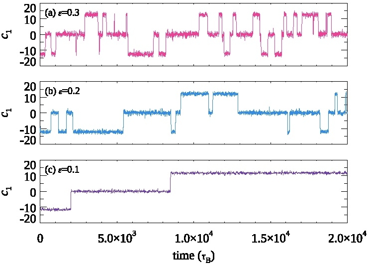
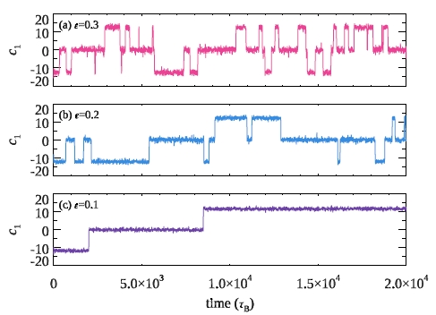
This is Fig. 7 from Weeks & Criddle, PRE 102, 062153 (2020). On the lab Linux computers, you can make this with IDL> @setup04 IDL> @mkfig04 Comments: This example makes it clear that your graphs can have any aspect ratio you might want. In terms of the POSITION graphics keyword, each graph has a width of 0.6 and a height of 0.2. I like how panels the panels are labeled "(a) epsilon = 0.3" so that the reader immediately knows the epsilon value without having to consult the caption. In hindsight, a missed opportunity: I should have made the middle panel purple and the bottom blue (as the bottom panel is the "coldest" behavior).

Extra tips

• I often use Coyote Graphics System's "symcat" to make interesting symbols (or better yet, the updated version cgSymCat). These IDL programs are installed on the lab linux computers.
• In general, using techniques from the Coyote Graphics website will greatly improve what you're doing. I haven't yet learned many of them.
• One example: I do some fancy stuff to pull in my desired rainbow of colors. If you prefer, use cgColor:

  IDL> color = cgPickColorName();  displays list of color names!
  IDL> plot,x,y,color=cgColor('Navy');   specify colors by name!
  IDL> oplot,a,b,color=cgColor('Steel Blue')
  

• A generally useful tip is to familiarize yourself with the graphics keywords. You don't need to memorize them, but knowing that they exist -- and some sense of what they can do -- can help you later. Like, if you need to turn the axes off, it's helpful to recall that you saw that somewhere in one of the graphics keywords even if you don't recall it's specifically XSTYLE and YSTYLE.