Eric Weeks
- personal pages - research
- time series analysis
My Adventures in Chaotic Time Series Analysis |
weeks@physics.emory.edu |
Eric Weeks
- personal pages - research
- time series analysis
My Adventures in Chaotic Time Series Analysis |
weeks@physics.emory.edu |
A0. Links and related information
For an explanation of what these pages are all about, select topic 1 above.
This page: top | lorenz | rossler | henon | expt: periodic | qperiodic-2 | qperiodic-3 | chaotic | bottom
![]()
The method of "mutual information" is a way to determine useful delay coordinates for plotting attractors.
The idea of delay coordinates is simple. If you can only observe one variable from a system, X(t), and you want to reconstruct a higher-dimensional attractor, you can consider (X(t),X(t+T),...,X(t+nT)) to produce a (n+1)-dimensional coordinate which can be plotted. It is important to choose a good value for T, the delay. If the delay is too short, then X(t) is very similar to X(t+T) and when plotted all of the data stays near the line X(t)=X(t+T). If the delay is too long, then the coordinates are essentially independent and no information can be gained from the plot. This can be seen in the next section.
The method of mutual information for finding the delay T was proposed
in an article by
Andrew M. Fraser and Harry L. Swinney ("Independent
coordinates for strange attractors from mutual information," Phys. Rev.
A 33 (1986) 1134-1140). The idea is that a good choice for T is one
that, given X(t), provides new information with measurement X(t+T).
To quote from the article, mutual information I is the answer to the
question, "Given a measurement of X(t), how many bits on the average can
be predicted about X(t+T)?" We want I(T) to be small. For more
information on information theory and this method, you should read the
article. Information theory is interesting stuff.
Practically speaking, the way this method works is to calculate I(T) for
a given time series. A graph of I(T) starts off very high (given a
measurement X(t), we know as many bits as possible about X(t+0)=X(t)).
As T is increased, I(T) decreases, then usually rises again. Fraser and
Swinney suggest using the first minimum in I(T) to select T.
Click here to get the program I wrote to calculate
the mutual information. Or, go to Fraser's home page
(above link) and get his original software, although I found
it a little more difficult to use.
Below I have the graphs of I(T) for my time series.
![]()
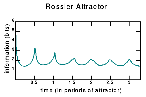
I did this one first as it's the test case that Fraser and Swinney use. Fortunately my graph resembles their graph, proving that I didn't make any mistakes writing the software. This graph has the x-axis shown in units of the natural period of the Rössler attractor. This period was determined from the Fourier transform of the data; see the previous section for a discussion. From this graph, the minimum is T=0.25 (times the period).
![]()
The first minimum occurs at T=0.16; the second slightly lower minimum occurs at T=0.62. In the next section you can see what the attractor looks like for these two choices.
![]()
This page:
top |
lorenz |
rossler |
henon |
expt: periodic |
qperiodic-2 |
qperiodic-3 |
chaotic |
bottom
Hénon:
time series
|
power spectrum
|
mutual information
|
attractor
|
attractor 3D
|
autocorrelation
|
poincare
|
1-D maps
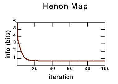
This graph looks much different, which is not suprising. For a simple map, the natural delay time is T=1 iteration. Given that the mutual information has no local minimum, but is only monotonically decreasing, this suggests that T=1 is a choice reasonably supported independently by the mutual information calculation.
![]()
This page:
top |
lorenz |
rossler |
henon |
expt: periodic |
qperiodic-2 |
qperiodic-3 |
chaotic |
bottom
Experimental/periodic:
time series
|
power spectrum
|
mutual information
|
attractor
|
attractor 3D
|
autocorrelation
|
poincare
|
1-D maps
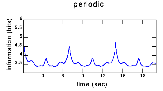
The first minimum occurs at 0.9 seconds; the second at 2.1 seconds. Recall that the for the periodic time series, the period was 6.9 seconds. The second maximum occurs at 3.5 s, about half the period.
![]()
This page:
top |
lorenz |
rossler |
henon |
expt: periodic |
qperiodic-2 |
qperiodic-3 |
chaotic |
bottom
Experimental/quasiperiodic-2:
time series
|
power spectrum
|
mutual information
|
attractor
|
attractor 3D
|
autocorrelation
|
poincare
|
1-D maps
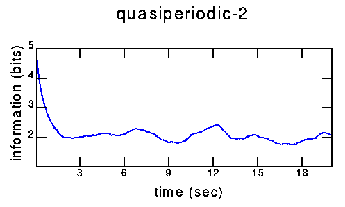
The first three minima occur at 2.5 s, 5.6 s, and 9.6 s. For this time series, the dominant period (as given by the Fourier transform) was 13 s. The first three maxima are at 4.8 s, 6.8 s (approximately half the period), and 12.3 s (close to one period).
![]()
This page:
top |
lorenz |
rossler |
henon |
expt: periodic |
qperiodic-2 |
qperiodic-3 |
chaotic |
bottom
Experimental/quasiperiodic-3:
time series
|
power spectrum
|
mutual information
|
attractor
|
attractor 3D
|
autocorrelation
|
poincare
|
1-D maps
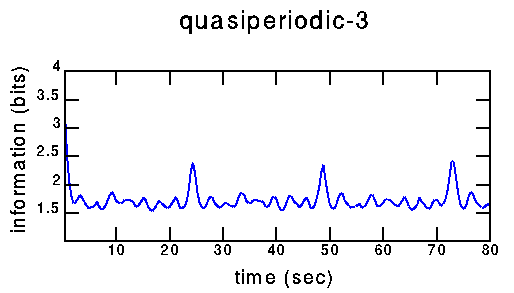
The first minimum is at 2.0 s, the second at 4.8 s. The largest peak in the power spectrum corresponds to a period of 6.1 s.
![]()
This page:
top |
lorenz |
rossler |
henon |
expt: periodic |
qperiodic-2 |
qperiodic-3 |
chaotic |
bottom
Experimental/chaotic:
time series
|
power spectrum
|
mutual information
|
attractor
|
attractor 3D
|
autocorrelation
|
poincare
|
1-D maps
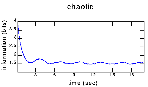
The first minimum is at 2.2 s. The first maximum is at 3.5 s. The natural period is 6.5 s.
![]()
So far the analysis has given me several different times. From the Fourier transform I have certain characteristic periods. From the mutual information calculation I have the first minimum. Thus, a table:
Note that all times are in natural units (seconds for experimental data, iterations for Hénon map, the time step of the equations for the Rössler and Lorenz systems). Links in the table will take you to the appropriate location where the information was found.
![]()
 Previous page: Fourier transforms
 Next page: Plotting the attractors
This page: top | lorenz | rossler | henon | expt: periodic | qperiodic-2 | qperiodic-3 | chaotic | bottom
![]()