 Click here to see the random walk page.
Work done by Eric Weeks, Tom Solomon, Jeff Urbach, and Harry Swinney. You may be interested in a paper we wrote for Nonlinear Science Today, which used to be an online-only journal, but which no longer exists. The article was intended for a broad audience and can be downloaded here: PDF format (2.5 MB).
This page maintained by Eric Weeks.
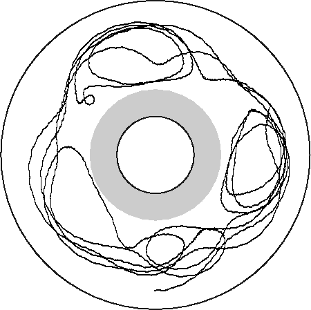
We study random walks of tracer particles in a rotating annulus. You might want to read the web page on random walks first. This page defines anomalous diffusion and discusses why it's interesting.
 Click here to see the random walk page.
 Click here to see a sketch of the rotating annulus experiment.
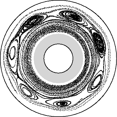
We follow small particles made from chopping up crayons in a rotating annulus. The flow consists of vortices and jets. The following picture is taken by following about 20 small particles for 90 s with a video camera and reconstructing the results on a computer. The camera is above the experiment, looking down. (We have studied flows with 4-7 vortices; the picture at the top of this web page is from a different flow than the one shown here.)
Individual particles alternately are trapped inside a vortex, and travel
long distances in the jet. We track individual particles by storing
the output of a video camera on a computer. The camera rotates
overhead. After the experiment is over, we use the stored information
to reconstruct where particles were each video frame, and by comparing
successive frames we track the individual particles. We can track about
50 particles simultaneously. (The gray circle in the middle of the picture,
and in the picture at the top of this web page, is a wall we inserted
into the experiment for technical reasons; in the pictures below
it appears as a dashed line..)
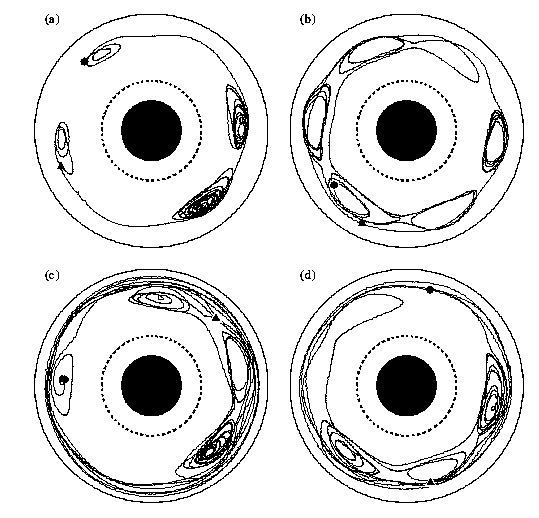
Below are some typical particle trajectories. The beginning of each trajectory is marked with a circle, the end with a triangle.
This is a graph of the angular coordinate, theta, as a function of time for the particle trajectory at the top of this web page.
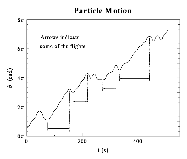
Notice that the particles are stuck for random lengths of times in the vortices, and travel for random lengths of time in the jets. Particles can travel in both directions in the jets. Thus, the motion of the particles is a random walk with random step sizes.
If you have read the random walks information page, or if you are familiar with anomalous diffusion, you are aware that the important question is how rare are the long flights. In particular, we are wondering how the probability of a long flight scales with the length.
We compile statistics on the motion of about 4000 particles to determine the probability of taking flights of various lengths. We also find the probability of being stuck inside a vortex for different times. (In our case, particles in the jet move with roughly constant velocity, so flight lengths are the same as flight times.) We find the following probability distribution functions (A, on the left, is for flights; B, on the right, is for sticking in a vortex).
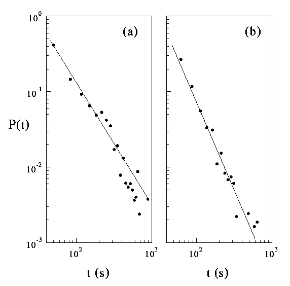
These are a log-log plot of probability -vs- flight and sticking times. The slope of the flight plot is -2.3, indicating that long flights of duration T occur with a probability proportional to T^(-2.2). This is the necessary and sufficient condition for these random walks to be Lévy flights. This is the first experiment where the Lévy flights of tracer particles can be seen directly with a camera, and their distributions measured from their actual motions.
The slope of the sticking plot is -1.6, thus the probability of being stuck in a vortex for a duration T is proportional to T^(-1.6).
By examining the behavior of all of the particles, it is possible to measure the variance and see directly how it grows in time. The variance in this case is defined by:
variance = < theta^2 > - < theta >^2
where the angle brackets < > mean averaging over all of the particles. Theta is the angular distance a particle has moved at a given point in time, so the formula defines the variance at that given point in time.
When we measure the variance, we get the following result (a log-log plot again):
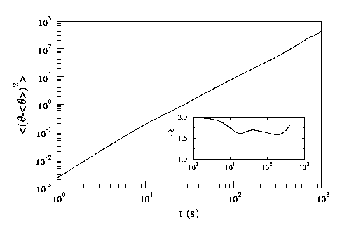
The inset shows the slope of this log-log plot as a function of time. For a reasonable period of time, the slope is approximately 1.65. This means that the variance is growing proportional to T^1.65, that is, faster than T^1.0, which means that the variance is growing superdiffusively.
If you read the random walks theory page, at the bottom of the page a specific prediction was made for the growth of the variance as a function of time, based on the behavior of the flight and sticking distribution functions. The specific prediction from theory (given that mu=2.2 and nu=1.6 as discussed above for the flight and sticking time behaviors respectively) is that the variance should grow as T^1.3 -- superdiffusively. The measured value is 1.65, superdiffusive but somewhat faster.
It is likely that the discrepancy is because we are unable to track particles for long enough times. The theory predicts the growth of the variance as time gets very large (goes to infinity), whereas we can only follow particles for times up to 1000 s.
This work is discussed in the following three papers: